

In this article, I will attempt to address the Input Embedding and Positional Encoding sections of the Transformers architecture.
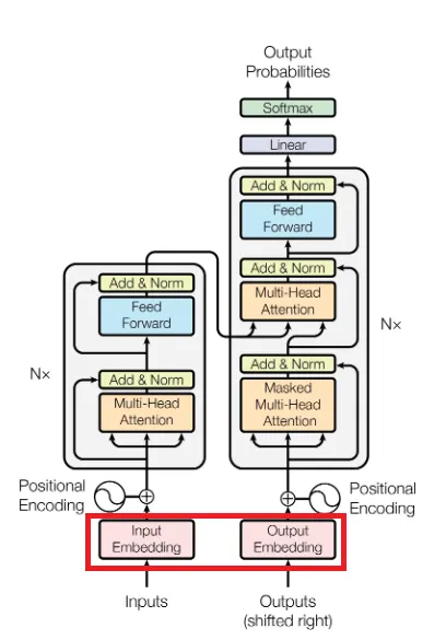
Let's try to understand the architecture step by step. Before moving on to the concept of Input Embedding, let's try to understand what Input is. Simply put, Input is the input text we give to the model. Of course, it is possible to train with different data types, but we will give our examples based on text data.

Above, we see an example sentence that will be input into our model. Our model cannot understand text as it is; we need to convert this text into numerical representations and feed our model in this way. Therefore, we first tokenize the sentences, meaning we break them down into words or smaller pieces (often tokenization is performed in different ways rather than word by word). The example text above has been tokenized word by word. After tokenization, we need to convert these words into numerical representations. We map words to numbers, and these numbers represent their positions in our vocabulary. Imagine we have a vocabulary consisting of all possible words that appear in our training set; each word will have a position in this vocabulary. For example, the word “cat” might occupy the 3578th position.
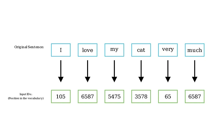
After the tokenization process described above, each word is represented by a number based on its position in the vocabulary. These numbers, or InputIDs, are mapped to a 512-dimensional vector. (This vector size varies depending on the model architecture.)
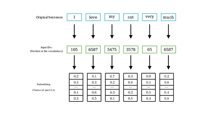
These 512-dimensional vectors are called embeddings. The same word is always mapped to the same InputID and embedding. However, the embedding numbers are not fixed; they are parameters for our model. Our model learns to change these numbers to represent meaning. As a result, the InputID values remain constant because the vocabulary is fixed, but the embeddings will change during the training process according to the needs of the loss function.
Note: Random numbers have been assigned to the embedding vectors in the images.
It may seem a bit confusing, but you understand the general idea. Input texts are split into pieces, numbers are assigned according to their positions, and these numbers are converted into another 512-dimensional vector. These converted 512-dimensional vectors are fed into our model as input, and calculations are performed on this matrix. In other words, the texts are converted into numerical representations.
When we talk about text data, you may be wondering: if the input is text, how can the model perform operations on texts of different sizes?
Variable-Length Sentences Padding
Since sentences vary in length, we need to set a maximum length to feed our model, and we need to add padding to words shorter than this maximum length to bring them up to the maximum length. This process is called padding.
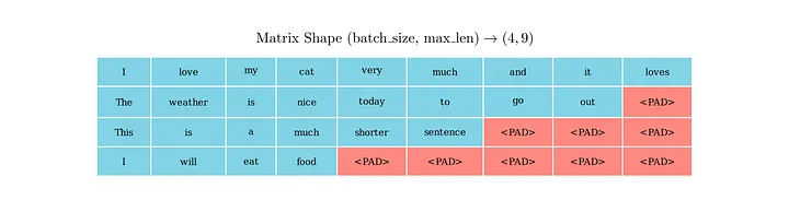
Let's assume we set the maximum input length of our model to 9. We add a <PAD> token to inputs shorter than 9 words to adjust their size to 9 words. This way, texts of variable length can be fed into our model as input with padding applied to reach the specified maximum length.

As a result, the input to our Transformer model becomes the 6x512 matrix shown above.
The maximum number of words our model will take as input is 6, and the embedding dimension is 512.
Positional Encoding
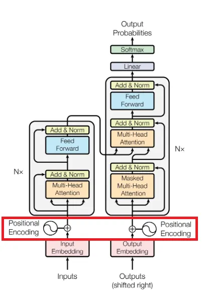
We have covered the concepts of Inputs and Input Embedding. Now let's try to understand the concept of Positional Encoding.
We have created a word matrix consisting of embeddings, but these embeddings do not carry any information about the position of a particular word within a sentence. This is where positional encoding comes into play.
We want the model to evaluate words that are close to each other as “close” and words that are far apart as “distant.” We need to ensure that the model sees this information as we perceive it with our eyes. For example, when we look at the sentence “what is positional encoding,” we understand that the word “what” is farther from the word ‘is’ than it is from the word “encoding.” This is because we can perceive this specific positional information with our eyes. However, the model cannot see this directly, so we need to provide the model with additional information about how the words are positioned within the sentence.
How is Positional Encoding Calculated?
Now that we understand why we need a positional encoding layer, let's try to understand how positional encoding is calculated and added to our input embedding matrix.

Positional Encoding is calculated according to the above formulas.
pos = the position of the word, for example, the word “cat” in the input text is in the 3rd position in the sentence. (The position index starts from 0)
i = 512-dimensional embedding vector index information
d_model = embedding vector size, which will be 512 in our example.
The concepts of 2i and 2i+1 ensure that calculations are performed using the cosine formula for single i values and the sine formula for double i values. I will explain later why we use two formulas, sine and cosine. For now, let's just keep in mind that cosine is used for single embedding index values and sine is used for double values.

As seen above, a positional encoding value is calculated for each word embedding value.
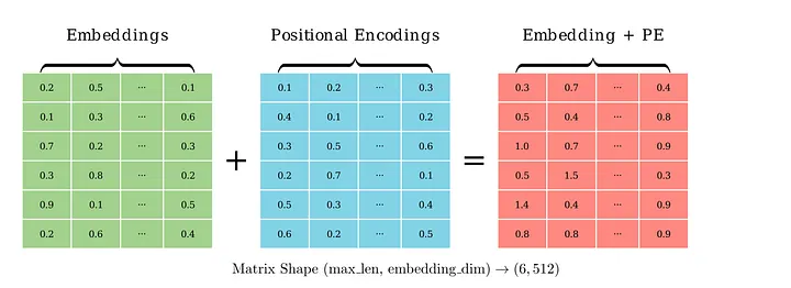
Then, the embedding matrix and the positional encoding matrix are added together to form our embedding matrix with the position information of the words added. Since we are adding matrices, the dimension remains unchanged and we preserve our initial dimension. We can pass this resulting matrix to the other steps of the architecture.
The positional encoding matrix is created once. The same matrix is used for training and inference because position information is a fixed value and the matrix does not change when the embedding changes, so the same position encoding matrix is added to different embedding matrices. We do not need to recalculate it every time we feed the model with new data.
Why Trigonometric Functions?
Sine and cosine functions are used because they provide a continuous and differentiable method for encoding position information. Their periodic nature enables the model to learn effectively and generalize across different positions, and their alternative uses across dimensions help preserve unique encodings for each position.
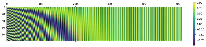
Above, we see a visualization of the positional encoding matrix with a maximum input size of 100 and an embedding size of 512. The sine and cosine functions have created a pattern at different positions, which we as humans can recognize, and we hope the model can understand it too.
Conclusion
In this article, I tried to explain the concepts of Input Embedding and Positional Encoding to understand how Transformer models work. I hope it has been useful for you as well. In the next article, we will discuss how the Multi-Head Attention mechanism is calculated using our matrix with Positional Encoding information.
Resources:
- Vaswani, A., Shazeer, N., Parmar, N., Uszkoreit, J., Jones, L., Gomez, A. A., Kaiser, Ł., & Polosukhin, I. (2017). Attention is all you need. arXiv. https://doi.org/10.48550/arXiv.1706.03762
- Jamil, U. “ Attention is all you need (Transformer) — Model explanation (including math), Inference and Training.” YouTube, uploaded by Umar Jamil, 28 May. 2023, https://www.youtube.com/watch?v=bCz4OMemCcA&t=1216s.
- GeeksforGeeks. (2024, May 15). Positional encoding in transformers. GeeksforGeeks. https://www.geeksforgeeks.org/positional-encoding-in-transformers/
- Saeed, M. (2023, January 6). A gentle introduction to positional encoding in transformer models – part 1. Machine Learning Mastery. https://machinelearningmastery.com/a-gentle-introduction-to-positional-encoding-in-transformer-models-part-1/
- Sammani, F. (2021). The Complete Neural Networks Bootcamp: Theory, Applications. Udemy. https://www.udemy.com/course/the-complete-neural-networks-bootcamp-theory-applications/
- Oluşturmuş olduğum görsellerin Manim Kodları, https://github.com/KaganHanCatan/Embedding-PositionalEncoding-Manim-Components
Author:


Orbislabs AI 2026. All Rights Reserved.


